Scene Flow

Scene flow denotes the real 3-D motion of objects in the scene, as opposed to optical flow, which only describes the projection of this motion on the 2-D image plane. In contrast to structure from motion, where a single camera moves through a static environment, scene flow does not relate to a rigid world, but objects are allowed to move around freely and deform in a non-rigid fashion. Since depth information is required to determine the 3-D motion of objects, scene flow can not be computed without estimating the scene structure as well. Unlike the stereo reconstruction problem, scene flow estimation has a temporal component and stereo sequences are needed that provide at least two views per time instance.

Applications of scene flow computation can be found in motion capture, dynamic rendering and vehicle navigation. In our work we have developed an algorithm that is purely image based and does not require any special hardware such as structured light or time-of-flight cameras. Because our approach is based on highly accurate variational optical flow estimation, we do not need to make explicit assumptions on the type of motion and are even able to obtain excellent results for small image sizes.

Reconstruction and scene flow	Scene flow vector plot	Scene flow color coded

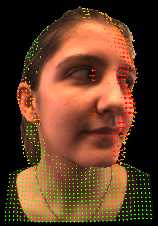
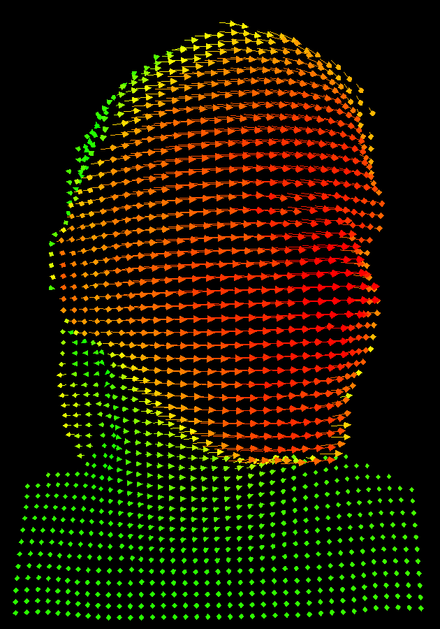
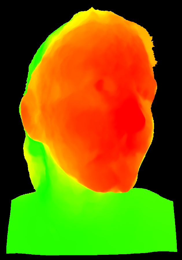
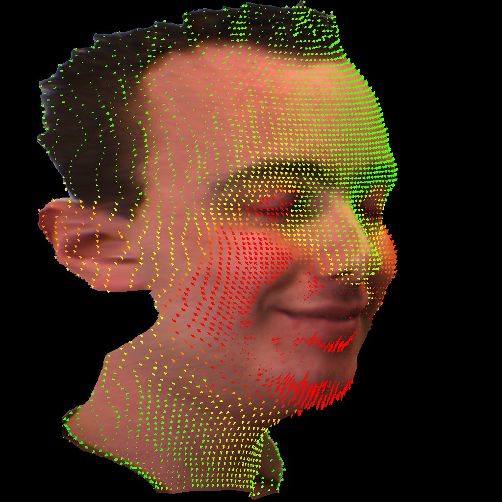
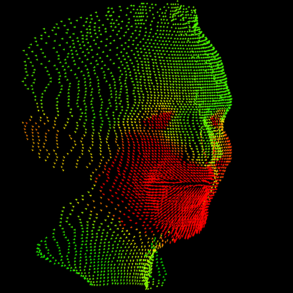
The figure shows an example of a model turning her head (click on the figures to enlarge). The left image shows the 3D reconstruction with the scene flow field superimposed as a vector plot. The flow vectors are colour coded depending on their magnitude: green indicates no or only small motion and red indicates large motion. The middle image only shows the scene flow vector field, while the right image depicts the magnitude of the scene flow in each point of the reconstructed surface.

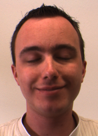
In [1] we compute the scene flow by considering the four-frame case depicted below. It consists of two consecutive image pairs of a synchronised stereo sequence: the left and the right image at a time instance t and the left and right image at time t+1. For our application we assume a fixed stereo rig, i.e. there exists a single fundamental matrix that describes the epipolar geometry of both stereo pairs. In the case of arbitrarily moving cameras, however, our model can also be generalised to a temporally varying fundamental matrix .



All together, we consider four types of correspondences in our model: two optical flows between consecutive frames in time and two stereo flows between the left and right frame at the same time instance. Furthermore, there is the unknown fundamental matrix, which restricts points in the left and right images to lie on corresponding epipolar lines. It can be demonstrated that this forms a complete parameterisation of the camera geometry, the scene structure and the three-dimensional scene motion. Similar to the optical flow method of Valgaerts et al. for partially calibrated stereo, we solve for all unknowns simultaneously. This ensures a maximal coupling between the optical flow (scene motion), the stereo flow (scene structure), and the epipolar geometry (camera motion).


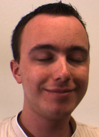
The above figure shows an example of a model closing his eyes and smiling (click on the figures to enlarge). The top row shows the left and right image at time t and the left and right image at time t + 1. The bottom row shows the 3D reconstruction with the scene flow field superimposed and the scene flow vector field.

1. L. Valgaerts, A. Bruhn, H. Zimmer, J. Weickert, C. Stoll, C. Theobalt:
   Joint Estimation of Motion, Structure and Geometry from Stereo Sequences.
   In Computer Vision - ECCV 2010, Proc. 11th European Conference on Computer Vision
   ECCV 2010, Heraklion, Greece, September 2010 - Kostas Daniilidis, Petros Maragos and Nikos Paragios (Eds.) Lecture Notes in Computer Science, Vol.6314, Springer, Berlin, 568-581, 2010.
   © Springer-Verlag Berlin Heidelberg 2010.
   
   See also:Supplementary Material Webpage.